
This is a small tutorial to illustrate how to simulate data from a variety of Sequential Sampling Models (SSMs) using the ssms python package.
The main simulators in this package are written in cython, to optimize for speed of computation.
SSMs?
SSMs take a central role in the joint modeling of reaction times and choice in Cognitive Science.
The ssms package is part of the hddm ecosystem to which, amongst others, the kabuki and lanfactory python packages belong.
It takes it’s place in this ecosystem, by providing the simulation backend for hddm package. Future blog-posts are going to complete this picture (and more), however for now note that ssms is useful in it’s own right.
Installation Instructions (colab)
Colab notebooks usually have quite a few packages preinstalled. It should be sufficient to simply install the ssms package.
# !pip install git+https://github.com/AlexanderFengler/ssms@main
Import Modules
import ssms
import pandas as pd
import numpy as np
import os
from matplotlib import pyplot as plt
Basic Package Outline
Let’s take a quick look at the structure of the ssms package by using the help functoin.
help(ssms)
Help on package ssms:

NAME
    ssms

PACKAGE CONTENTS
    basic_simulators (package)
    config (package)
    dataset_generators (package)
    support_utils (package)

VERSION
    0.2.0

FILE
    /users/afengler/data/software/miniconda3/envs/pymc_ak_lan/lib/python3.9/site-packages/ssms/__init__.py
The package consists of four main submodules.
- The
basic_simulatorssubmodule, which provides low level access to the model simulators. - The
configsubmodule provides configuration files for the models included. - The
dataset_generatorssubmodule builds on top of thebasic_simulatorsmodule and supplies a variety of methods for systematically generating data for downstream usecases. This is biased towards generating training data for usage with thelanfactorypackage. Thelanfactorypackage in turn feeds into thehddmpackage with compatible neural network classes. Learn more about what the goals behind this pipeline are here and here. - The
support_utilsmodule collect a few convenience functions that may be helpful when usingssms.
Background on the modeling framework
Let’s simulate some data from the basic Diffusion Decision Model (DDM).
We can use the ssms.config.model_config dictionary to check some information about this model. Importantly we can check the number, name (and order) of parameters under the 'params' keyword. In this case there are four parameters, ['v', 'a', 'z', 't'].
ssms.config.model_config['ddm']
{'name': 'ddm',
 'params': ['v', 'a', 'z', 't'],
 'param_bounds': [[-3.0, 0.3, 0.1, 0.0], [3.0, 2.5, 0.9, 2.0]],
 'boundary': <function ssms.basic_simulators.boundary_functions.constant(t=0)>,
 'n_params': 4,
 'default_params': [0.0, 1.0, 0.5, 0.001],
 'hddm_include': ['z'],
 'nchoices': 2}
There is a large literature applying the DDM for the analysis of reaction time and choice data from a large variety of behavioral and/or psychophysics experiments. You can learn more about the interpretation of these parameters e.g. here.
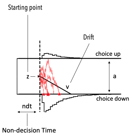
Shortly, the Diffusion Decision Model assumes that decision and reactions times derive from boundary crossings of a particle diffusion process. The parameters then have the following interpretations:
- ‘v’ is a deterministic drift applied to the particle over time (one interpretation is that this describes the rate of evidence accumulation over time).
- ‘a’ is the height of the boundary to be crossed (crossing the upper or lower boundary respectively describe unique choices).
- ‘z’ is the starting point of the particle (which may be biased towards either boundary, in turn representing choice options).
- ‘t’ accounts for the part of a final reaction time captured by all processes unrelated to the actual processing of the decision-relevant evidence. It simply shifts the final decision time.
The picture below illustrates. Note, the upper and lower black histograms describe the reaction time distributions for the upper and lower choice respectively.
Let’s simulate
from ssms.basic_simulators import simulator
Using the simulator() function we can pick our model of choice (model argument), supply a vector (or matrix for a trial-wise logic on parameter values) of parameters and set a number of n_samples we want to draw from our DDM process. The delta_t arguments controls how fine-grained the time-steps of our simulator are. Interpret $0.001$ as timesteps of $1ms$. Making the time-steps coarser, will speed up the simulation however reduce the accuracy with which the underlying diffusion process is represented by the simulations.
ssms uses the basic Euler Maruyama method to forward simulate the diffusion trajectories (particle trajectories).
simulations = simulator(model = 'ddm',
                        theta = [1., 1.5, 0.5, 0.5],
                        n_samples = 1000,
                        delta_t = 0.001,
                        random_state = 42)
The output of the simulator function is python dictionary, with three keys.
rtsstoring the simulated reaction times. Values are positive real numbers.choicesstoring the respective choices. Values are-1,1respectively for lower and upper boundary crossings.metadatastores information about the simulator configurations and more.
simulations.keys()
dict_keys(['rts', 'choices', 'metadata'])
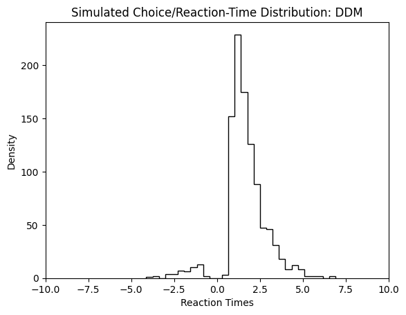
A simple way to plot the resulting simulator runs is to put negative choices (the lower bound was crossed) on the negative real numbers, and positive choices on the positive real numbers, then using a simple histogram to illustrate the total (choice, reaction-time) - distribution.
plt.hist(simulations['rts'] * simulations['choices'],
         bins = 30,
         histtype = 'step',
         color = 'black')
plt.xlim(-10, 10)
plt.xlabel("Reaction Times")
plt.ylabel("Density")
plt.title("Simulated Choice/Reaction-Time Distribution: DDM")
plt.show()
Changing the Model
Instead we might be interested in simulating from a model of the following form.
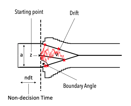
We can check the properties of this model via the ssms.config.model_config dictionary again. This time under the angle, key.
ssms.config.model_config['angle']
{'name': 'angle',
 'params': ['v', 'a', 'z', 't', 'theta'],
 'param_bounds': [[-3.0, 0.3, 0.1, 0.001, -0.1], [3.0, 3.0, 0.9, 2.0, 1.3]],
 'boundary': <function ssms.basic_simulators.boundary_functions.angle(t=1, theta=1)>,
 'n_params': 5,
 'default_params': [0.0, 1.0, 0.5, 0.001, 0.0],
 'hddm_include': ['z', 'theta'],
 'nchoices': 2}
The parameters are equivalent to the DDM models’, however the theta parameter is added, which specifies the angle of the boundaries.
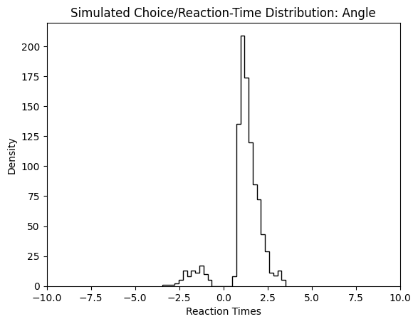
simulations_angle = simulator(model = 'angle',
                        theta = [1., 1.5, 0.5, 0.5, 0.3],
                        n_samples = 1000,
                        delta_t = 0.001,
                        random_state = 42)
plt.hist(simulations_angle['rts'] * simulations_angle['choices'],
         bins = 30,
         histtype = 'step',
         color = 'black')
plt.xlim(-10, 10)
plt.xlabel("Reaction Times")
plt.ylabel("Density")
plt.title("Simulated Choice/Reaction-Time Distribution: Angle")
plt.show()
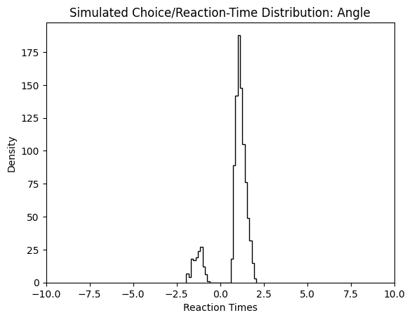
We can change to value of the theta parameter, and observe how the simulated reaction times change in response.
simulations_angle = simulator(model = 'angle',
                        theta = [1., 1.5, 0.5, 0.5, 0.7],
                        n_samples = 1000,
                        delta_t = 0.001,
                        random_state = 42)
plt.hist(simulations_angle['rts'] * simulations_angle['choices'],
         bins = 30,
         histtype = 'step',
         color = 'black')
plt.xlim(-10, 10)
plt.xlabel("Reaction Times")
plt.ylabel("Density")
plt.title("Simulated Choice/Reaction-Time Distribution: Angle")
plt.show()
How to investigate the ready-to-use models
ssms comes with a large variety of such model variations predefined. As mentioned above, you can learn about them by inspecting the model_config dictionary.
Few basic principles may help you navigate the space of the models. Take another example, the model corresponding to the "weibull", key.
ssms.config.model_config['weibull']
{'name': 'weibull',
 'params': ['v', 'a', 'z', 't', 'alpha', 'beta'],
 'param_bounds': [[-2.5, 0.3, 0.2, 0.001, 0.31, 0.31],
  [2.5, 2.5, 0.8, 2.0, 4.99, 6.99]],
 'boundary': <function ssms.basic_simulators.boundary_functions.weibull_cdf(t=1, alpha=1, beta=1)>,
 'n_params': 6,
 'default_params': [0.0, 1.0, 0.5, 0.001, 3.0, 3.0],
 'hddm_include': ['z', 'alpha', 'beta'],
 'nchoices': 2}
To understand the properties of this model look for the following attributes.
- The
v,a,z,tparameters have essentially equivalent interpretations across the board (see above). - The
boundaryis eitherNoneor afunction, which is vectorized along thetinput (for time). The argument names to the function correspond to the names in theparams,key. Here, thealphaandbetaarguments refer to boundary parameters. - The
nchoices,keycontains the number of choice options that a given model allows. To interpret model behavior, there are essentially two kinds of settings. Eithernchoicesis set to2, in which case the model can be interpreted as simulating a single particle which moves between two (upper and lower) boundaries. Ifnchoices > 2, then we should interpret the model as have as many moving particles, which cross a single upper bound.
Let’s take a look at the boundary of the "weibull" model.
from ssms.basic_simulators.boundary_functions import weibull_cdf

plt.plot(np.linspace(0, 1, 1000),
         weibull_cdf(t = np.linspace(0, 10, 1000), alpha = 1.5, beta = 3),
         color = 'black')
plt.plot(np.linspace(0, 1, 1000),
         -weibull_cdf(t = np.linspace(0, 10, 1000), alpha = 1.5, beta = 3),
         color = 'black')
plt.ylim(-1.1, 1.1)
plt.xlim(0, 1)
plt.title("weibull_cdf() boundary")
plt.xlabel("Time in seconds")
plt.ylabel("Boundary Value")
plt.show()
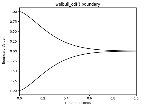
There are two styles or boundaries: multiplicative and additive.
If the boundary function automatically gives you boundary values between $0$ and $1$, then the boundary will be multiplicative, meaning that the a parameters will be multiplied by the boundary shape to get the final boundary applied in the simulator. Else, a will be added to the boundary returned by the given bounadry function.
Hence, the weibull_cdf() boundary is multiplicative.
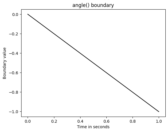
In contrast consider the angle() boundary.
from ssms.basic_simulators.boundary_functions import angle

plt.plot(np.linspace(0, 1, 1000),
         angle(t = np.linspace(0, 10, 1000), theta = 0.1),
         color = 'black')
plt.title("angle() boundary")
plt.xlabel("Time in seconds")
plt.ylabel("Boundary value")
plt.show()
Timings
from time import time
n_samples = 1000
time_start = time()
for i in range(10):
    simulations_angle = simulator(model = 'ddm',
                                  theta = [1., 1.5, 0.5, 0.5],
                                  n_samples = n_samples,
                                  delta_t = 0.001,
                                  random_state = 42)
time_end = time()

print('The simulator ran an average of ', round((time_end - time_start) / 10, 2), 'seconds \nto produce', n_samples, 'sample trajectories from the DDM!')
The simulator ran an average of  0.09 seconds
to produce 1000 sample trajectories from the DDM!
End
Stay tuned for a sequence of blog posts, which will close the gap (via the lanfactory package) towards using the hddm and finally the pymc python package for purposes of hierarchical bayesian modeling (inference) with such SSMs.
We will learn more about ssms, specifically how to leverage the package to generate training data for jax (with the help of the flax and optax packages) and pytorch networks. We will then consider training such networks conveniently with the lanfactory package.
Such neural networks can then be used as likelihood functions for bayesian inference with hddm and/or pymc, following recent research in computational cognitive science. We will motivate why one may be interested in this approach to inference.